Grassmann.jl

⟨Grassmann-Clifford-Hodge⟩ multilinear differential geometric algebra

The Grassmann.jl package provides tools for computations based on multi-linear algebra and spin groups using the extended geometric algebra known as Grassmann-Clifford-Hodge algebra. Algebra operations include exterior, regressive, inner, and geometric, along with the Hodge star and boundary operators. Code generation enables concise usage of the algebra syntax. DirectSum.jl multivector parametric type polymorphism is based on tangent vector spaces and conformal projective geometry. Additionally, the universal interoperability between different sub-algebras is enabled by AbstractTensors.jl, on which the type system is built. The design is based on TensorAlgebra{V} abstract type interoperability from AbstractTensors.jl with a K-module type parameter V from DirectSum.jl. Abstract vector space type operations happen at compile-time, resulting in a differential geometric algebra of multivectors.

   ____  ____    ____   _____  _____ ___ ___   ____  ____   ____
  /    T|    \  /    T / ___/ / ___/|   T   T /    T|    \ |    \
 Y   __j|  D  )Y  o  |(   \_ (   \_ | _   _ |Y  o  ||  _  Y|  _  Y
 |  T  ||    / |     | \__  T \__  T|  \_/  ||     ||  |  ||  |  |
 |  l_ ||    \ |  _  | /  \ | /  \ ||   |   ||  _  ||  |  ||  |  |
 |     ||  .  Y|  |  | \    | \    ||   |   ||  |  ||  |  ||  |  |
 l___,_jl__j\_jl__j__j  \___j  \___jl___j___jl__j__jl__j__jl__j__j

This Grassmann package for the Julia language was created by github.com/chakravala for mathematics and computer algebra research with differential geometric algebras. These projects and repositories were started entirely independently and are available as free software to help spread the ideas to a wider audience. Please consider donating to show your thanks and appreciation to this project at liberapay, GitHub Sponsors, Patreon, Tidelift, Bandcamp or contribute (documentation, tests, examples) in the repositories.

• Requirements
• DirectSum.jl parametric type polymorphism
• Grassmann.jl API design overview
• Visualization examples
• References

TensorAlgebra{V} design and code generation

Mathematical foundations and definitions specific to the Grassmann.jl implementation provide an extensible platform for computing with a universal language for finite element methods based on a discrete manifold bundle. Tools built on these foundations enable computations based on multi-linear algebra and spin groups using the geometric algebra known as Grassmann algebra or Clifford algebra. This foundation is built on a DirectSum.jl parametric type system for tangent bundles and vector spaces generating the algorithms for local tangent algebras in a global context. With this unifying mathematical foundation, it is possible to improve efficiency of multi-disciplinary research using geometric tensor calculus by relying on universal mathematical principles.

• AbstractTensors.jl: Tensor algebra abstract type interoperability setup
• DirectSum.jl: Tangent bundle, vector space and Submanifold definition
• Grassmann.jl: ⟨Grassmann-Clifford-Hodge⟩ multilinear differential geometric algebra

using Grassmann, Makie; @basis S"∞+++"
streamplot(vectorfield(exp((π/4)*(v12+v∞3)),V(2,3,4),V(1,2,3)),-1.5..1.5,-1.5..1.5,-1.5..1.5,gridsize=(10,10))

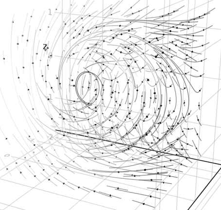
More information and tutorials are available at https://grassmann.crucialflow.com/dev

Requirements

Grassmann.jl is a package for the Julia language, which can be obtained from their website or the recommended method for your operating system (GNU/Linux/Mac/Windows). Go to docs.julialang.org for documentation. Availability of this package and its subpackages can be automatically handled with the Julia package manager using Pkg; Pkg.add("Grassmann") or

pkg> add Grassmann

If you would like to keep up to date with the latest commits, instead use

pkg> add Grassmann#master

which is not recommended if you want to use a stable release. When the master branch is used it is possible that some of the dependencies also require a development branch before the release. This may include, but not limited to:

This requires a merged version of ComputedFieldTypes at https://github.com/vtjnash/ComputedFieldTypes.jl

Interoperability of TensorAlgebra with other packages is enabled by DirectSum.jl and AbstractTensors.jl.

The package is compatible via Requires.jl with Reduce.jl, Symbolics.jl, SymPy.jl, SymEngine.jl, AbstractAlgebra.jl, GaloisFields.jl, LightGraphs.jl, UnicodePlots.jl, Makie.jl, GeometryBasics.jl, Meshes.jl,

Sponsor this at liberapay, GitHub Sponsors, Patreon, or Bandcamp, Tidelift, Tidelift (Learn more).

DirectSum.jl parametric type polymorphism

The AbstractTensors package is intended for universal interoperation of the abstract TensorAlgebra type system. All TensorAlgebra{V} subtypes have type parameter V, used to store a Submanifold{M} value, which is parametrized by M the TensorBundle choice. This means that different tensor types can have a commonly shared underlying K-module parametric type expressed by defining V::Submanifold{M}. Each TensorAlgebra subtype must be accompanied by a corresponding TensorBundle parameter, which is fully static at compile time. Due to the parametric type system for the K-module types, the compiler can fully pre-allocate and often cache.

Let V be a K-module of rank n be specified by instance with the tuple (n,P,g,ν,μ) with P specifying the presence of the projective basis and g is a metric tensor specification. The type TensorBundle{n,P,g,ν,μ} encodes this information as byte-encoded data available at pre-compilation, where μ is an integer specifying the order of the tangent bundle (i.e. multiplicity limit of the Leibniz-Taylor monomials). Lastly, ν is the number of tangent variables, bases for the vectors and covectors; and bases for differential operators and scalar functions. The purpose of the TensorBundle type is to specify the K-module basis at compile time. When assigned in a workspace, V = Submanifold(::TensorBundle).

The metric signature of the Submanifold{V,1} elements of a vector space V can be specified with the V"..." by using + or - to specify whether the Submanifold{V,1} element of the corresponding index squares to +1 or -1. For example, S"+++" constructs a positive definite 3-dimensional TensorBundle, so constructors such as S"..." and D"..." are convenient.

It is also possible to change the diagonal scaling, such as with D"1,1,1,0", although the Signature format has a more compact representation if limited to +1 and -1. It is also possible to change the diagonal scaling, such as with D"0.3,2.4,1". Fully general MetricTensor as a type with non-diagonal components requires a matrix, e.g. MetricTensor([1 2; 2 3]).

Declaring an additional point at infinity is done by specifying it in the string constructor with ∞ at the first index (i.e. Riemann sphere S"∞+++"). The hyperbolic geometry can be declared by ∅ subsequently (i.e. hyperbolic projection S"∅+++"). Additionally, the null-basis based on the projective split for conformal geometric algebra would be specified with S"∞∅+++". These two declared basis elements are interpreted in the type system. The tangent(V,μ,ν) map can be used to specify μ and ν.

To assign V = Submanifold(::TensorBundle) along with associated basis elements of the DirectSum.Basis to the local Julia session workspace, it is typical to use Submanifold elements created by the @basis macro,

julia> using Grassmann; @basis S"-++" # macro or basis"-++"
(⟨-++⟩, v, v₁, v₂, v₃, v₁₂, v₁₃, v₂₃, v₁₂₃)

the macro @basis V delcares a local basis in Julia. As a result of this macro, all Submanifold{V,G} elements generated with M::TensorBundle become available in the local workspace with the specified naming arguments. The first argument provides signature specifications, the second argument is the variable name for V the K-module, and the third and fourth argument are prefixes of the Submanifold vector names (and covector names). Default is V assigned Submanifold{M} and v is prefix for the Submanifold{V}.

It is entirely possible to assign multiple different bases having different signatures without any problems. The @basis macro arguments are used to assign the vector space name to V and the basis elements to v..., but other assigned names can be chosen so that their local names don’t interfere: If it is undesirable to assign these variables to a local workspace, the versatile constructs of DirectSum.Basis{V} can be used to contain or access them, which is exported to the user as the method DirectSum.Basis(V).

julia> DirectSum.Basis(V)
DirectSum.Basis{⟨-++⟩,8}(v, v₁, v₂, v₃, v₁₂, v₁₃, v₂₃, v₁₂₃)

V(::Int...) provides a convenient way to define a Submanifold by using integer indices to reference specific direct sums within ambient V.

Additionally, a universal unit volume element can be specified in terms of LinearAlgebra.UniformScaling, which is independent of V and has its interpretation only instantiated by context of TensorAlgebra{V} elements being operated on. Interoperability of LinearAlgebra.UniformScaling as a pseudoscalar element which takes on the TensorBundle form of any other TensorAlgebra element is handled globally. This enables the usage of I from LinearAlgebra as a universal pseudoscalar element defined at every point x of a manifold, which is mathematically denoted by I = I(x) and specified by the g(x) bilinear tensor field.

Grassmann.jl API design overview

Grassmann.jl is a foundation which has been built up from a minimal K-module algebra kernel on which an entirely custom algbera specification is designed and built from scratch on the base Julia language.

Definition. TensorAlgebra{V,K} where V::Submanifold{M} for a generating K-module specified by a M::TensorBundle choice

• TensorBundle specifies generators of DirectSum.Basis algebra
  • Int value induces a Euclidean metric of counted dimension
  • Signature uses S"..." with + and - specifying the metric
  • DiagonalForm uses D"..." for defining any diagonal metric
  • MetricTensor can accept non-diagonal metric tensor array
• TensorGraded{V,G,K} has grade G element of exterior algebra
  • Chain{V,G,K} has a complete basis for grade G with K-module
  • Simplex{V} alias column-module Chain{V,1,Chain{V,1,K}}
• TensorTerm{V,G,K} <: TensorGraded{V,G,K} single coefficient
  • Zero{V} is a zero value which preserves V in its algebra type
  • Submanifold{V,G,B} is a grade G basis with sorted indices B
  • Single{V,G,B,K} where B::Submanifold{V} is paired to K
• AbstractSpinor{V,K} subtypes are special Clifford sub-algebras
  • Couple{V,B,K} is the sum of K scalar with Single{V,G,B,K}
  • PseudoCouple{V,B,K} is pseudoscalar + Single{V,G,B,K}
  • Spinor{V,K} has complete basis for the even Z2-graded terms
  • CoSpinor{V,K} has complete basis for odd Z2-graded terms
• Multivector{V,K} has complete exterior algebra basis with K-module

Definition. TensorNested{V,T} subtypes are linear transformations

• TensorOperator{V,W,T} linear operator mapping with T::DataType
  • Endomorphism{V,T} linear endomorphism map with T::DataType
• DiagonalOperator{V,T} diagonal endomorphism with T::DataType
  • DiagonalMorphism{V,<:Chain{V,1}} diagonal map on grade 1 vectors
  • DiagonalOutermorphism{V,<:Multivector{V}} on full exterior algebra
• Outermorphism{V,T} extends Endomorphism{V} to full exterior algebra
• Projector{V,T} linear map with F(F) = F defined
• Dyadic{V,X,Y} linear map with Dyadic(x,y) = x ⊗ y

Grassmann.jl was first to define a comprehensive TensorAlgebra{V} type system from scratch around the idea of the V::Submanifold{M} value to express algebra subtypes for a specified K-module structure.

Definition. Common unary operations on TensorAlgebra elements

• Manifold returns the parameter V::Submanifold{M} K-module
• mdims dimensionality of the pseudoscalar V of that TensorAlgebra
• gdims dimensionality of the grade G of V for that TensorAlgebra
• tdims dimensionality of Multivector{V} for that TensorAlgebra
• grade returns G for TensorGraded{V,G} while grade(x,g) is selection
• istensor returns true for TensorAlgebra elements
• isgraded returns true for TensorGraded elements
• isterm returns true for TensorTerm elements
• complementright Euclidean metric Grassmann right complement
• complementleft Euclidean metric Grassmann left complement
• complementrighthodge Grassmann-Hodge right complement reverse(x)*I
• complementlefthodge Grassmann-Hodge left complement I*reverse(x)
• metric applies the metricextensor as outermorphism operator
• cometric applies complement metricextensor as outermorphism
• metrictensor returns g bilinear form associated to TensorAlgebra{V}
• metrictextensor returns outermorphism form for TensorAlgebra{V}
• involute grade permutes basis per k with grade(x,k)*(-1)^k
• reverse permutes basis per k with grade(x,k)*(-1)^(k(k-1)/2)
• clifford conjugate of an element is composite involute ∘ reverse
• even part selects (x + involute(x))/2 and is defined by even grade
• odd part selects (x - involute(x))/2 and is defined by odd grade
• real part selects (x + reverse(x))/2 and is defined by positive square
• imag part selects (x - reverse(x))/2 and is defined by negative square
• abs is the absolute value sqrt(reverse(x)*x) and abs2 is then reverse(x)*x
• norm evaluates a positive definite norm metric on the coefficients
• unit applies normalization defined as unit(t) = t/abs(t)
• scalar selects grade 0 term of any TensorAlgebra element
• vector selects grade 1 terms of any TensorAlgebra element
• bivector selects grade 2 terms of any TensorAlgebra element
• trivector selects grade 3 terms of any TensorAlgebra element
• pseudoscalar max. grade term of any TensorAlgebra element
• value returns internal Values tuple of a TensorAlgebra element
• valuetype returns type of a TensorAlgebra element value’s tuple

Binary operations commonly used in Grassmann algebra syntax

• + and - carry over from the K-module structure associated to K
• wedge is exterior product ∧ and vee is regressive product ∨
• > is the right contraction and < is the left contraction of the algebra
• * is the geometric product and / uses inv algorithm for division
• ⊘ is the sandwich and >>> is its alternate operator orientation

Custom methods related to tensor operators and roots of polynomials

• inv returns the inverse and adjugate returns transposed cofactor
• det returns the scalar determinant of an endomorphism operator
• tr returns the scalar trace of an endomorphism operator
• transpose operator has swapping of row and column indices
• compound(F,g) is the graded multilinear Endomorphism
• outermorphism(A) transforms Endomorphism into Outermorphism
• operator make linear representation of multivector outermorphism
• companion matrix of monic polynomial a0 + a1*z + ... + an*z^n + z^(n+1)
• roots(a...) of polynomial with coefficients a0 + a1*z + ... + an*z^n
• rootsreal of polynomial with coefficients a0 + a1*z + ... + an*z^n
• rootscomplex of polynomial with coefficients a0 + a1*z + ... + an*z^n
• monicroots(a...) of monic polynomial a0 + a1*z + ... + an*z^n + z^(n+1)
• monicrootsreal of monic polynomial a0 + a1*z + ... + an*z^n + z^(n+1)
• monicrootscomplex of monic polynomial a0 + a1*z + ... + an*z^n + z^(n+1)
• characteristic(A) polynomial coefficients from det(A-λ*I)
• eigvals(A) are the eigenvalues [λ1,...,λn] so that A*ei = λi*ei
• eigvalsreal are real eigenvalues [λ1,...,λn] so that A*ei = λi*ei
• eigvalscomplex are complex eigenvalues [λ1,...,λn] so A*ei = λi*ei
• eigvecs(A) are the eigenvectors [e1,...,en] so that A*ei = λi*ei
• eigvecsreal are real eigenvectors [e1,...,en] so that A*ei = λi*ei
• eigvecscomplex are complex eigenvectors [e1,...,en] so A*ei = λi*ei
• eigen(A) spectral decomposition sum of λi*Proj(ei) with A*ei = λi*ei
• eigenreal spectral decomposition sum of λi*Proj(ei) with A*ei = λi*ei
• eigencomplex spectral decomposition sum of λi*Proj(ei) so A*ei = λi*ei
• eigpolys(A) normalized symmetrized functions of eigvals(A)
• eigpolys(A,g) normalized symmetrized function of eigvals(A)
• vandermonde facilitates (inv(X'X)*X')*y for polynomial coefficients
• cayley(V,∘) returns product table for V and binary operation ∘

Accessing metrictensor(V) produces a linear map g which can be extended to an outermorphism given by metricextensor. To apply the metricextensor to any Grassmann element, the function metric can be used on the element, cometric applies a complement metric.

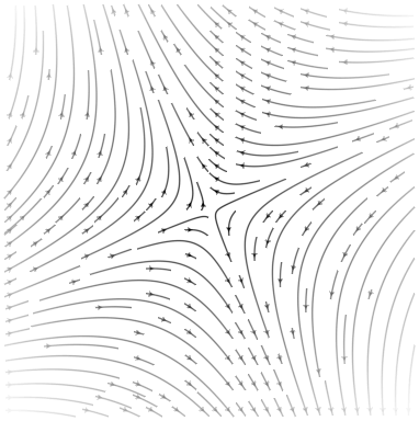
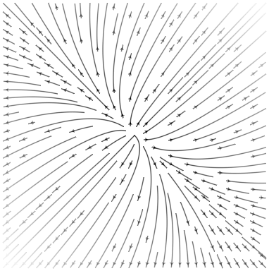
Visualization examples

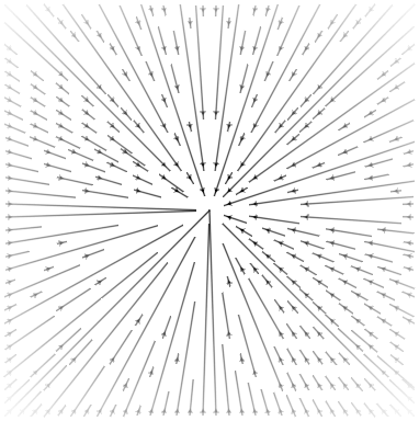
Due to GeometryBasics.jl Point interoperability, plotting and visualizing with Makie.jl is easily possible. For example, the vectorfield method creates an anonymous Point function that applies a versor outermorphism:

using Grassmann, Makie
basis"2" # Euclidean
streamplot(vectorfield(exp(π*v12/2)),-1.5..1.5,-1.5..1.5)
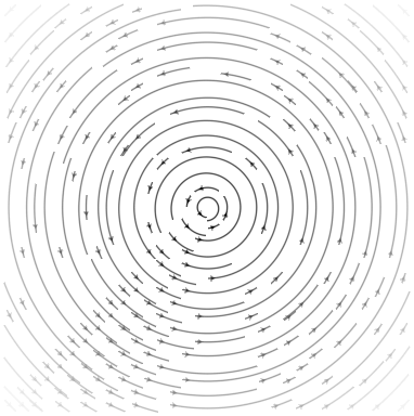
streamplot(vectorfield(exp((π/2)*v12/2)),-1.5..1.5,-1.5..1.5)
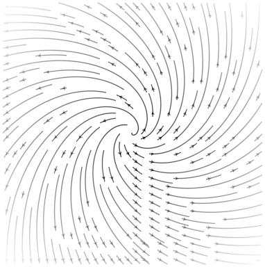
streamplot(vectorfield(exp((π/4)*v12/2)),-1.5..1.5,-1.5..1.5)
streamplot(vectorfield(v1*exp((π/4)*v12/2)),-1.5..1.5,-1.5..1.5)
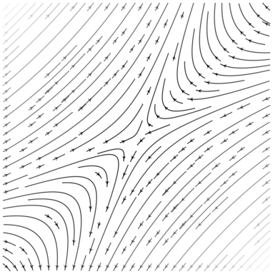
@basis S"+-" # Hyperbolic
streamplot(vectorfield(exp((π/8)*v12/2)),-1.5..1.5,-1.5..1.5)
streamplot(vectorfield(v1*exp((π/4)*v12/2)),-1.5..1.5,-1.5..1.5)

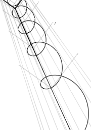
using Grassmann, Makie
@basis S"∞+++"
f(t) = (↓(exp(π*t*((3/7)*v12+v∞3))>>>↑(v1+v2+v3)))
lines(V(2,3,4).(points(f)))
@basis S"∞∅+++"
f(t) = (↓(exp(π*t*((3/7)*v12+v∞3))>>>↑(v1+v2+v3)))
lines(V(3,4,5).(points(f)))

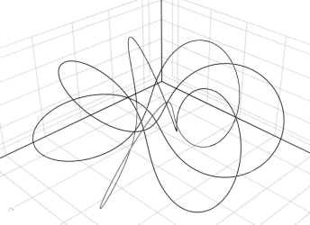
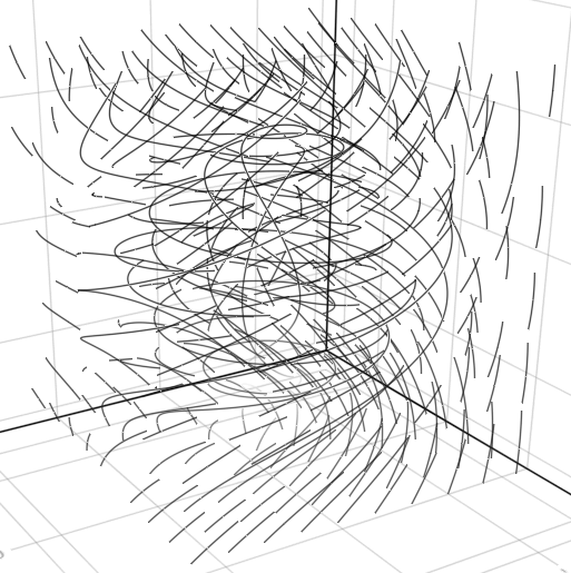
using Grassmann, Makie; @basis S"∞+++"
streamplot(vectorfield(exp((π/4)*(v12+v∞3)),V(2,3,4)),-1.5..1.5,-1.5..1.5,-1.5..1.5,gridsize=(10,10))

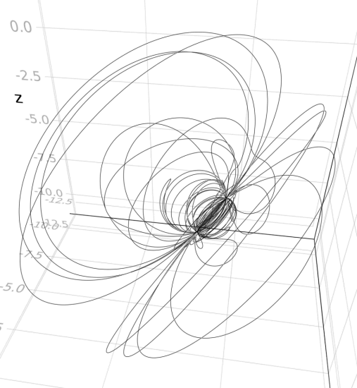
using Grassmann, Makie; @basis S"∞+++"
f(t) = ↓(exp(t*v∞*(sin(3t)*3v1+cos(2t)*7v2-sin(5t)*4v3)/2)>>>↑(v1+v2-v3))
lines(V(2,3,4).(points(f)))

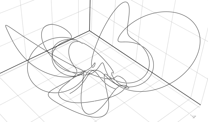
using Grassmann, Makie; @basis S"∞+++"
f(t) = ↓(exp(t*(v12+0.07v∞*(sin(3t)*3v1+cos(2t)*7v2-sin(5t)*4v3)/2))>>>↑(v1+v2-v3))
lines(V(2,3,4).(points(f)))

References

• Michael Reed, Differential geometric algebra with Leibniz and Grassmann, JuliaCon (2019)
• Michael Reed, Foundatons of differential geometric algebra (2021)
• Michael Reed, Multilinear Lie bracket recursion formula (2024)
• Michael Reed, Differential geometric algebra: compute using Grassmann.jl and Cartan.jl (2025)
• Emil Artin, Geometric Algebra (1957)
• John Browne, Grassmann Algebra, Volume 1: Foundations (2011)
• C. Doran, D. Hestenes, F. Sommen, and N. Van Acker, Lie groups as spin groups, J. Math Phys. (1993)
• David Hestenes, Universal Geometric Algebra, Pure and Applied (1988)
• David Hestenes, Renatus Ziegler, Projective Geometry with Clifford Algebra, Acta Appl. Math. (1991)
• David Hestenes, Tutorial on geometric calculus. Advances in Applied Clifford Algebra (2013)
• Lachlan Gunn, Derek Abbott, James Chappell, Ashar Iqbal, Functions of multivector variables (2011)
• Aaron D. Schutte, A nilpotent algebra approach to Lagrangian mechanics and constrained motion (2016)
• Vladimir and Tijana Ivancevic, Undergraduate lecture notes in DeRahm-Hodge theory. arXiv (2011)
• Peter Woit, Clifford algebras and spin groups, Lecture Notes (2012)

This site is open source. Improve this page.