Grassmann elements and geometric algebra Λ(V)

Definition (Vector space $\Lambda^1 V = V$ is a field's $\mathbb K$-module instance). Let $V$ be a $\mathbb K$-module (abelian group with respect to $+$) with an element $1\in\mathbb K$ such that $1V = V$ by scalar multiplication $\mathbb K\times V\rightarrow V$ over field $\mathbb K$ satisfying

1. $a(x+y) = ax+ ay$ distribution of vector addition,
2. $(a+b)x = ax + bd$ distribution of field addition,
3. $(ab)x = a(bx)$ associative compatibility.

In the software package Grassmann, a generating vector space $\mathbb{K}$-module is specified as a value of <:TensorBundle (an abstract type).

Definition (Linear dependence). Let $V$ be a vector space over field $\mathbb K$, then the set $\{v_i\}_i$ is linearly dependent if and only if $\sum_{i=1}^n k_iv_i = 0$ for some $0\ne k\in\mathbb K^n$.

Definition ($\wedge$-product annihilation). For a linearly dependent set $\{v_i\}_1^n\subset V$

\[v_1\wedge v_2\wedge\dots\wedge v_n = 0.\]

Initially, it is enough to understand that $\wedge:\Lambda^n V\times\Lambda^m V\rightarrow\Lambda^{n+m}V$ is an operation which is zero for linearly dependent arguments. However, this idea comes from extending Grassmann's product $v_i\wedge v_j = -v_j\wedge v_i \implies v_i\wedge v_i = 0 = -v_i\wedge v_i$ to yield a tool for characterizing linear dependence.

Definition (Dimension $n$-Submanifold in $\Lambda^n V$). Note that writing the product $v_1\wedge v_2\wedge\cdots\wedge v_n\ne0$ implies a linearly independent set $\{v_i\}_1^n\subseteq V$ isomorphic to an $n$-Submanifold.

Furthermore, $\mathbb{K}\times\{v_1\wedge v_2\wedge\cdots\wedge v_n\}\cong\mathbb{K}$ shows the $1$-dimensional basis subspace is induced by any $n$-Submanifold.

Example. Therefore, $\mathbb K = \Lambda^0\mathbb K \cong \Lambda^1\mathbb K$ is a vector space or a 0-Submanifold.

Example. $\Lambda^n V$ is a vector space with $\Lambda^1\Lambda^n V = \Lambda^nV$ and $\Lambda^0\Lambda^nV = \Lambda^0V$.

Denote $V^* = V\backslash\{0\}$ as the set $V$ excluding the 0 element in next:

Definition (Direct sum $\oplus$). To consider a set of linearly independent spaces, let $\pi_i: V\rightarrow V_i$ be projections with vector space $V_i\subset V$, define

\[V_1\oplus V_2\oplus\cdots\oplus V_n = V \iff \bigwedge : V_1^*\times V_2^*\times\cdots\times V_n^* \rightarrow \Lambda^n V^* .\]

DirectSum of a full non-zero product implies an $n$-Submanifold.

Ddefinition Grade-$m$ projection is defined as $\langle\Lambda V\,\rangle_m = \Lambda^m V$ such that

\[\Lambda V = \bigoplus_{m=0}^n \langle\Lambda V\,\rangle_m = \Lambda^0V\oplus\Lambda^1V\oplus\cdots\oplus\Lambda^nV, \qquad \langle\Lambda V\,\rangle_m = \bigoplus_{m=1}^{n\choose m}\mathbb K.\]

Note that $\dim \langle\Lambda V\,\rangle_m = {n\choose m}$ and hence $\dim\Lambda V = \sum_{m=0}^n {n\choose m} = 2^n$.

Example (Combinatorics of power set $\mathcal P(V)$). Let $v_1,v_2,v_3 \in\mathbb R^3$, then the power set of elements is:

\[\mathcal P(\mathbb R^3) = \{\emptyset,\{v_1\},\{v_2\},\{v_3\},\{v_1,v_2\},\{v_1,v_3\},\{v_2,v_3\},\{v_1,v_2,v_3\}\}\]

Form a direct sum over the elements of $\mathcal P(V)$ with $\wedge$ to define $\Lambda V$, e.g.

\[\Lambda(\mathbb R^3) = \Lambda^0(\mathbb R^3)\oplus\Lambda^1(\mathbb R^3)\oplus\Lambda^2(\mathbb R^3)\oplus\Lambda^3(\mathbb R^3)\]

\[\overbrace{v_\emptyset}^{\Lambda^0\mathbb R}\oplus \overbrace{v_1\oplus v_2\oplus v_3}^{\Lambda^1(\mathbb R^3)}\oplus\overbrace{(v_1\wedge v_2)\oplus (v_1\wedge v_3) \oplus (v_2\wedge v_3)}^{\Lambda^2(\mathbb R^3)}\oplus\overbrace{(v_1\wedge v_2\wedge v_3)}^{\Lambda^3(\mathbb R^3)}\]

The Grassmann Submanifold elements $v_k\in\Lambda^1V$ and $w^k\in\Lambda^1V'$ are linearly independent vector and covector elements of $V$, while the Leibniz Operator elements $\partial_k\in L^1V$ are partial tangent derivations and $\epsilon_k\in L^1V'$ are dependent functions of the tangent manifold. Let $V\in\text{Vect}_{\mathbb k}$ be a TensorBundle with dual space $V'$ and the basis elements $w_k:V\rightarrow\mathbb K$, then for all $x\in V,c\in\mathbb K$ it holds: $(w^i+w^j)(x) = w^i(x)+w^j(x)$ and $(cw^k)(x) = cw^k(x)$ hold. An element of a mixed-symmetry TensorAlgebra{V} is a multilinear mapping that is formally constructed by taking the tensor products of linear and multilinear maps, $(\bigotimes_k \omega_k)(v_1,\dots,v_{\sum_k p_k}) = \prod_k \omega_k(v_1,\dots,v_{p_k})$. Higher grade elements correspond to Submanifold subspaces, while higher order function elements become homogenous polynomials and Taylor series.

julia> Λ(ℝ^3)DirectSum.Basis{⟨+++⟩,8}(v, v₁, v₂, v₃, v₁₂, v₁₃, v₂₃, v₁₂₃)
julia> Λ(tangent(ℝ^2))DirectSum.Basis{T¹⟨++₁⟩,8}(v, v₁, v₂, ∂₁, v₁₂, ∂₁v₁, ∂₁v₂, ∂₁v₁₂)
julia> Λ(tangent((ℝ^0)',3,3))DirectSum.Basis{T³⟨¹²³⟩',8}(w, ϵ₁, ϵ₂, ϵ₃, ϵ₁₂, ϵ₁₃, ϵ₂₃, ϵ₁₂₃)

Combining the linear basis generating elements with each other using the multilinear tensor product yields a graded (decomposable) tensor Submanifold $\langle v_{i_1}\otimes\cdots\otimes v_{i_k}\rangle_k : V'^k\rightarrow\mathbb K$, where rank is determined by the sum of basis index multiplicities in the tensor product decomposition. The Grassmann anti-symmetric exterior basis is denoted by $v_{i_1\dots i_g}\in\Lambda^gV$ having the dual elements $w^{i_1\cdots i_g}\in\Lambda^gV'$, while the Leibniz symmetric basis will be denoted by $\partial_{i_1}^{\mu_1}\dots\partial_{i_g}^{\mu_g}\in L^gV$ with corresponding $\epsilon_{i_1}^{\mu_1}\dots\epsilon_{i_g}^{\mu_g}\in L^gV'$ adjoint elements. Combined, this space produces the full Leibniz tangent algebra $T^\mu V=V\oplus (\bigoplus_{g=1}^\mu L^g V)$ and the Grassmann exterior algebra $\Lambda V = \bigoplus_{g=1}^n\Lambda^g V$ with $2^n$ elements. The mixed index algebra $\Lambda(T^\mu V) = (\bigoplus_{g=1}^n\Lambda^g V)\oplus(\bigoplus_{g=1}^\mu L^g V)$ is partitioned into both symmetric and anti-symmetric tensor equivalence classes. Any mixed tensor Submanifold pair $\omega,\eta$ satisfies either

\[\underbrace{\omega\otimes\eta = -\eta\otimes\omega}_{\text{anti-symmetric}} \qquad \text{or} \qquad \underbrace{\omega\otimes\eta = \eta\otimes\omega}_{\text{symmetric}}.\]

For the oriented sets of the Grassmann exterior algebra, the parity of $(-1)^\Pi$ is factored into transposition compositions when interchanging ordering of the tensor product argument permutations. The symmetrical algebra does not need to track this parity, but has higher multiplicities in its indices. Symmetric differential function algebra of Leibniz trivializes the orientation into a single class of index multi-sets, while Grassmann's exterior algebra is partitioned into two oriented equivalence classes by anti-symmetry. Full tensor algebra can be sub-partitioned into equivalence classes in multiple ways based on the element symmetry, grade, and metric signature composite properties. Both symmetry classes can be characterized by the same geometric product.

julia> indices(Λ(3).v12)2-element Vector{Int64}:
 1
 2

A higher-order composite tensor element is an oriented-multi-set $X$ such that $v_X = \bigotimes_k v_{i_k}^{\otimes\mu_k}$ with the indices $X = \left((i_1,\mu_1),\dots,(i_g,\mu_g)\right)$ and $|X|=\sum_k\mu_k$ is tensor rank. Anti-symmetric indices $\Lambda X\subseteq\Lambda V$ have two orientations and higher multiplicities of them result in zero values, so the only interesting multiplicity is $\mu_k\equiv1$. The Leibniz-Taylor algebra is a quotient polynomial ring $LV\cong R[x_1,\dots,x_n]/\{\prod_{k=1}^{\mu+1} x_{p_k}\}$ so that $\partial_k^{\mu+1}$ is zero. Typically the $k$ in a product $\left(\partial_{p_1}\otimes\cdots\otimes\partial_{p_k}\right)^{(k)}$ is referred to as the order of the element if it is fully symmetric, which is overall tracked separately from the grade such that $\partial_k\langle v_j\rangle_r = \langle\partial_kv_j\rangle_r$ and $(\partial_k)^{(r)}\omega_j = (\partial_kv_j)^{(r)}$. There is a partitioning into even grade components $\omega_+$ and odd grade components $\omega_-$ such that $\omega_++\omega_-=\omega$.

Grassmann's exterior algebra doesn't invoke the properties of multi-sets, as it is related to the algebra of oriented sets; while the Leibniz symmetric algebra is that of unoriented multi-sets. Combined, the mixed-symmetry algebra yield a multi-linear propositional lattice. The formal sum of equal grade elements is an oriented Chain and with mixed grade it is a Multivector simplicial complex. Thus, various standard operations on the oriented multi-sets are possible including $\cup,\cap,\oplus$ and the index operation $\ominus$, which is symmetric difference operation.

Grassmann's exterior product is an anti-symmetric tensor product

\[v_i \wedge v_j = - v_j\wedge v_i \implies v_i\wedge v_i = 0 = -v_i\wedge v_i,\]

which generalizes the multilinear determinant transposition property

\[v_{\omega_1}\wedge\cdots\wedge v_{\omega_m}\wedge v_{\eta_1}\wedge\cdots\wedge v_{\eta_n} = (-1)^{mn} v_{\eta_1} \wedge \cdots \wedge v_{\eta_n} \wedge v_{\omega_1} \wedge \cdots \wedge v_{\omega_m}.\]

Hence for graded elements it is possible to deduce that

\[\omega \in \Lambda^mV,\quad\eta\in\Lambda^nV : \qquad \omega\wedge\eta = (-1)^{mn}\eta\wedge\omega.\]

Remark. Observe the anti-symmetry property implies that $\omega\otimes\omega = 0$, while the symmetric property neither implies nor denies such a property.

Example. Case of 3rd order tangent bundle operators composition:

\[T^3(\Lambda^0V) = \partial_\emptyset \oplus \partial_1\oplus\partial_2\oplus\partial_3 \oplus (\partial_1\circ\partial_2) \oplus (\partial_1\circ\partial_3) \oplus (\partial_2\circ\partial_3) \oplus (\partial_1\circ\partial_2\circ\partial_3)\]

In order to shorten the notation, the operation symbol is left out:

\[\{v_1,v_2,v_3,v_{12},v_{13},v_{23},v_{123}\}, \{\partial_1,\partial_2,\partial_3,\partial_{12},\partial_{13},\partial_{23},\partial_{123}\}\]

The canonical choice of orientation is with indices in sorted order, so that for example anti-symmetry is applied to rewrite $v_{21} = -v_{12}$ or the property $\partial_2\circ\partial_1 = \partial_1\circ\partial_2$ is applied for differential operators. In general, permutations of the indices get rendered as orientations of $(-1)^k$ of a basis $\mathbb{K}$-module.

Definition (Permutations). Consider $\displaystyle\sigma_j(\omega) = \sum_{k=0}^n(-1)^{\binom{k}{2^{j-1}}}\langle\omega\rangle_k$,

\[\sigma_1(\omega) \equiv \overline\omega, \qquad \sigma_2(\omega) \equiv \widetilde\omega, \qquad \sigma_{12} = \sigma_2(\sigma_1(\omega)) \equiv \widetilde{\overline{\omega}}\]

Theorem ($\mathfrak{S}_j = \langle\sigma_1,\sigma_2,\dots,\sigma_j\rangle$ is a group). $\mathfrak{S}_2 = \{1,\sigma_1,\sigma_2,\sigma_{12}\}$ is a set of automorphisms: grade involution $\overline\omega = \sigma_1(\omega) = \sum_{k=0}^n (-1)^{\binom{k}{1}}\langle\omega\rangle_k$, reverse $\widetilde\omega = \sigma_2(\omega) = \sum_{k=0}^n (-1)^{\binom{k}{2}}\langle\omega\rangle_k = \sum_{k=0}^n (-1)^{(k-1)k/2}\langle\omega\rangle_k$ is an anti-automorphism with $\sigma_2(v_i\wedge v_j) = \sigma_2(v_j)\wedge\sigma_2(v_i)$, and Clifford conjugate $\widetilde{\overline\omega}$ is the composition of grade involution and reverse anti-automorphism.

Definition (Real $\widetilde{\mathfrak{R}}\omega = (\omega + \widetilde\omega)/2$ and imaginary $\widetilde{\mathfrak{I}}\omega = (\omega - \widetilde\omega)/2$). Real and imaginary define $\mathbb{Z}_2$-grading projections so that $\Lambda V = \widetilde{\mathfrak{R}}\Lambda V \oplus \widetilde{\mathfrak{I}}\Lambda V$; where $\widetilde{\mathfrak{R}}\Lambda V$ is the real part and $\widetilde{\mathfrak{I}}\Lambda V$ is the imag (imaginary) part.

Definition (Even $\overline{\mathfrak{R}}\omega = (\omega + \overline\omega)/2$ and odd $\overline{\mathfrak{I}}\omega = (\omega - \overline\omega)/2$). Even and odd define $\mathbb{Z}_2$-grading projections so that $\Lambda V = \overline{\mathfrak{R}}\Lambda V \oplus \overline{\mathfrak{I}}\Lambda V$; where $\overline{\mathfrak{R}}\Lambda V$ is the even part and $\overline{\mathfrak{I}}\Lambda V$ is the odd part.

In general, this can be extended to $\mathbb{Z}_2$-grading projections $\sigma_j$ and its real $\sigma_j(\mathfrak{R})\omega = (\omega + \sigma_j(\omega))/2$ and imaginary $\sigma_j(\mathfrak{I})\omega = (\omega-\sigma_j(\omega))/2$ parts.

Grassmann.jl API design overview

Grassmann.jl is a foundation which has been built up from a minimal $\mathbb{K}$-module algebra kernel on which an entirely custom algbera specification is designed and built from scratch on the base Julia language.

Definition. TensorAlgebra{V,$\mathbb{K}$} where V::Submanifold{M} for a generating $\mathbb{K}$-module specified by a M::TensorBundle choice

• TensorBundle specifies generators of DirectSum.Basis algebra
  • Int value induces a Euclidean metric of counted dimension
  • Signature uses S"..." with + and - specifying the metric
  • DiagonalForm uses D"..." for defining any diagonal metric
  • MetricTensor can accept non-diagonal metric tensor array
• TensorGraded{V,G,$\mathbb{K}$} has grade $G$ and element of $\Lambda^GV$ subspace
  • Chain{V,G,$\mathbb{K}$} has a complete basis for $\Lambda^GV$ with $\mathbb{K}$-module
  • Simplex{V} alias column-module Chain{V,1,Chain{V,1,$\mathbb{K}$}}
• TensorTerm{V,G,$\mathbb{K}$} <: TensorGraded{V,G,$\mathbb{K}$} single coefficient
  • Zero{V} is a zero value which preserves $V$ in its algebra type
  • Submanifold{V,G,B} $\langle v_{i_1}\wedge\cdots\wedge v_{i_G}\rangle_G$ with sorted indices $B$
  • Single{V,G,B,$\mathbb{K}$} where B::Submanifold{V} is paired to $\mathbb{K}$
• AbstractSpinor{V,$\mathbb{K}$} subtypes are special sub-algebras of $\Lambda V$
  • Couple{V,B,$\mathbb{K}$} is the sum of $\mathbb{K}$ scalar with Single{V,G,B,$\mathbb{K}$}
  • PseudoCouple{V,B,$\mathbb{K}$} is pseudoscalar + Single{V,G,B,$\mathbb{K}$}
  • Spinor{V,$\mathbb{K}$} has complete basis for the even $\mathbb{Z}_2$-graded terms
  • CoSpinor{V,$\mathbb{K}$} has complete basis for odd $\mathbb{Z}_2$-graded terms
• Multivector{V,$\mathbb{K}$} has complete basis for all $\Lambda V$ with $\mathbb{K}$-module

Definition. TensorNested{V,T} subtypes are linear transformations

• TensorOperator{V,W,T} linear map $V\rightarrow W$ with T::DataType
  • Endomorphism{V,T} linear map $V\rightarrow V$ with T::DataType
• DiagonalOperator{V,T} diagonal map $V\rightarrow V$ with T::DataType
  • DiagonalMorphism{V,<:Chain{V,1}} diagonal map $V\rightarrow V$
  • DiagonalOutermorphism{V,<:Multivector{V}} $:\Lambda V\rightarrow \Lambda V$
• Outermorphism{V,T} extends $F\in$ Endomorphism{V} to full $\Lambda V$

\[F(v_1)\wedge\cdots\wedge F(v_n) = F(v_1\wedge\cdots\wedge v_n)\]

• Projector{V,T} linear map $F:V\rightarrow V$ with $F(F) = F$ defined

\[\verb`Proj(x::TensorGraded)` = \frac{x}{|x|}\otimes\frac{x}{|x|}\]

• Dyadic{V,X,Y} linear map $V\rightarrow V$ with Dyadic(x,y) $= x\otimes y$

Grassmann.jl was first to define a comprehensive TensorAlgebra{V} type system from scratch around the idea of the V::Submanifold{M} value to express algebra subtypes for a specified $\mathbb{K}$-module structure.

Definition. Common unary operations on TensorAlgebra elements

• Manifold returns the parameter V::Submanifold{M} $\mathbb{K}$-module
• mdims dimensionality of the pseudoscalar $V$ of that TensorAlgebra
• gdims dimensionality of the grade $G$ of $V$ for that TensorAlgebra
• tdims dimensionality of Multivector{V} for that TensorAlgebra
• grade returns $G$ for TensorGraded{V,G} while grade(x,g) is $\langle x\rangle_g$
• istensor returns true for TensorAlgebra elements
• isgraded returns true for TensorGraded elements
• isterm returns true for TensorTerm elements
• complementright Euclidean metric Grassmann right complement
• complementleft Euclidean metric Grassmann left complement
• complementrighthodge Grassmann-Hodge right complement $\widetilde\omega I$
• complementlefthodge Grassmann-Hodge left complement $I\widetilde\omega$
• metric applies the metricextensor as outermorphism operator
• cometric applies complement metricextensor as outermorphism
• metrictensor returns $g:V\rightarrow V$ associated to TensorAlgebra{V}
• metrictextensor returns $\Lambda g:\Lambda V\rightarrow\Lambda V$ for TensorAlgebra{V}
• involute grade permutes basis with $\langle\overline\omega\rangle_k = \sigma_1(\langle\omega\rangle_k) = (-1)^k\langle\omega\rangle_k$
• reverse permutes basis with $\langle\widetilde\omega\rangle_k = \sigma_2(\langle\omega\rangle_k) = (-1)^{k(k-1)/2}\langle\omega\rangle_k$
• clifford conjugate of an element is composite involute $\circ$ reverse
• even part selects $\overline{\mathfrak{R}}\omega = (\omega + \overline\omega)/2$ and is defined by $\Lambda^g$ for even $g$
• odd part selects $\overline{\mathfrak{I}}\omega = (\omega-\overline\omega)/2$ and is defined by $\Lambda^g$ for odd $g$
• real part selects $\widetilde{\mathfrak{R}}\omega = (\omega+\widetilde\omega)/2$ and is defined by $|\widetilde{\mathfrak{R}}\omega|^2 = (\widetilde{\mathfrak{R}}\omega)^2$
• imag part selects $\widetilde{\mathfrak{I}}\omega = (\omega-\widetilde\omega)/2$ and is defined by $|\widetilde{\mathfrak{I}}\omega|^2 = -(\widetilde{\mathfrak{I}}\omega)^2$
• abs is the absolute value $|\omega|=\sqrt{\widetilde\omega\omega}$ and abs2 is then $|\omega|^2 = \widetilde\omega\omega$
• norm evaluates a positive definite norm metric on the coefficients
• unit applies normalization defined as unit(t) = t/abs(t)
• scalar selects grade 0 term of any TensorAlgebra element
• vector selects grade 1 terms of any TensorAlgebra element
• bivector selects grade 2 terms of any TensorAlgebra element
• trivector selects grade 3 terms of any TensorAlgebra element
• pseudoscalar max. grade term of any TensorAlgebra element
• value returns internal Values tuple of a TensorAlgebra element
• valuetype returns type of a TensorAlgebra element value's tuple

Binary operations commonly used in Grassmann algebra syntax

• + and - carry over from the $\mathbb{K}$-module structure associated to $\mathbb{K}$
• wedge is exterior product $\wedge$ and vee is regressive product $\vee$
• > is the right contraction and < is the left contraction for $\Lambda V$
• * is the geometric product and / uses inv algorithm for division
• $\oslash$ is the sandwich and >>> is its alternate operator orientation

Custom methods related to tensor operators and roots of polynomials

• inv returns the inverse and adjugate returns transposed cofactor
• det returns the scalar determinant of an endomorphism operator
• tr returns the scalar trace of an endomorphism operator
• transpose operator has swapping of row and column indices
• compound(F,g) is multilinear endomorphism $\Lambda^gF : \Lambda^g V\rightarrow\Lambda^g V$
• outermorphism(A) transforms $A:V\rightarrow V$ into $\Lambda A:\Lambda V\rightarrow\Lambda V$
• operator make linear representation of multivector outermorphism
• companion matrix of monic polynomial $a_0+a_1z+\dots+a_nz^n + z^{n+1}$
• roots(a...) of polynomial with coefficients $a_0 + a_1z + \dots + a_nz^n$
• rootsreal of polynomial with coefficients $a_0 + a_1z + \dots + a_nz^n$
• rootscomplex of polynomial with coefficients $a_0 + a_1z + \dots + a_nz^n$
• monicroots(a...) of monic polynomial $a_0+a_1z+\dots+a_nz^n + z^{n+1}$
• monicrootsreal of monic polynomial $a_0+a_1z+\dots+a_nz^n + z^{n+1}$
• monicrootscomplex of monic polynomial $a_0+a_1z+\dots+a_nz^n + z^{n+1}$
• characteristic(A) polynomial coefficients from $\det (A-\lambda I)$
• eigvals(A) are the eigenvalues $[\lambda_1,\dots,\lambda_n]$ so that $A e_i = \lambda_i e_i$
• eigvalsreal are real eigenvalues $[\lambda_1,\dots,\lambda_n]$ so that $A e_i = \lambda_i e_i$
• eigvalscomplex are complex eigenvalues $[\lambda_1,\dots,\lambda_n]$ so $A e_i = \lambda_i e_i$
• eigvecs(A) are the eigenvectors $[e_1,\dots,e_n]$ so that $A e_i = \lambda_i e_i$
• eigvecsreal are real eigenvectors $[e_1,\dots,e_n]$ so that $A e_i = \lambda_i e_i$
• eigvecscomplex are complex eigenvectors $[e_1,\dots,e_n]$ so $A e_i = \lambda_i e_i$
• eigen(A) spectral decomposition $\sum_i \lambda_i\text{Proj}(e_i)$ with $A e_i = \lambda_i e_i$
• eigenreal spectral decomposition $\sum_i \lambda_i\text{Proj}(e_i)$ with $A e_i = \lambda_i e_i$
• eigencomplex spectral decomposition $\sum_i \lambda_i\text{Proj}(e_i)$ so $A e_i = \lambda_i e_i$
• eigpolys(A) normalized symmetrized functions of eigvals(A)
• eigpolys(A,g) normalized symmetrized function of eigvals(A)
• vandermonde facilitates $((X'X)^{-1} X')y$ for polynomial coefficients
• cayley(V,$\circ$) returns product table for $V$ and binary operation $\circ$

Accessing metrictensor(V) produces a linear map $g: V\rightarrow V$ which can be extended to $\Lambda g:\Lambda V\rightarrow\Lambda V$ outermorphism given by metricextensor. To apply the metricextensor to any Grassmann element of $\Lambda V$, the function metric can be used on the element, cometric applies a complement metric.

Grassmann-Hodge complement

John Browne has discussed the Grassmann duality principle, stating that every theorem (involving either of the exterior and regressive products) can be translated into its dual theorem by replacing the $\wedge$ and $\vee$ operations and applying Grassmann complements!

Definition (Grassmann $!$ complement). Expressed as unary operator, "right hand rule" is derived from John Browne's common factor theorem, given a pseudoscalar $\langle v_1\wedge\cdots\wedge v_n\rangle_n\in \Lambda^n V$ the linear map $!:\Lambda^mV \ra \Lambda^{n-m}V$

\[\langle v_{i_1}\wedge\cdots\wedge v_{i_m}\rangle_m \quad \mapsto \quad (-1)^{\frac{m(m+1)}{2} + \sum_{j=1}^m i_j} \langle\bigwedge_{k\ne i_j} v_k\rangle_{n-m},\]

also denoted as complementright for "right hand rule." While the linear inverse of $!$ is a similar map complementleft expressible by re-orientation:

\[\langle v_{i_1}\wedge\cdots\wedge v_{i_m}\rangle_m \quad \mapsto \quad (-1)^{m(n-1)}!\langle v_{i_1}\wedge\cdots\wedge v_{i_m}\rangle_m.\]

Together, these form an orthocomplementary propositional lattice $!,\wedge,\vee$

\[(!\bigvee_k\omega_k)(v_1,\dots,v_n) = (\bigwedge_k !\omega_k)(v_1,\dots,v_n) \quad DeMorgan's\,\,Law,\]

where the regressive product $\vee$ satisfies the Grassmann laws with $!$ and $\wedge$.

Definition (Hodge $\star$ complement). Expressed as unary operator $\star$, define the composition of $\star =$ complementright $\circ$ metric as linear operator.

\[\star ={!\Lambda g} : \Lambda V \rightarrow \Lambda V\]

This linear operator is also called complementrighthodge or only hodge.

Remark. Original Grassmann complement is equivalent to the Hodge complement with a Euclidean metric tensor, making metric an identity.

Definition. The interior contraction $\eta\cdot\omega = \eta\vee\star\omega$ is defined in terms of the regressive product and also the Hodge complement. By default the right contraction $>$ is used, but there is also a left contraction $<$ with swapped arguments $\eta<\omega = \omega\vee\star\eta$, and also $\eta >> \omega = \widetilde\eta >\omega$ with $\eta << \omega = \eta <\widetilde{\omega}$.

Remark. Using coupled subspaces in the block matrix structure of metric tensors, a basis element can be factorized in a corresponding way. In particular, for the diagonal metric this is simply the basis index factorization. However, a non-diagonal metric induces a more complex block factorization.

Definition (Clifford geometric product). If $a_i$ is an indecomposable basis element with regards to the block matrix structure of the metric tensor and $B\in\Lambda^kV$ is a graded element, then define operation $\ominus$ as either

\[ a_i\ominus B = a_i\wedge B + a_i<\widetilde B, \qquad B\ominus a_i = B\wedge a_i + \widetilde B>a_i\]

If $A = a_1\wedge\cdots\wedge a_m$ are a basis factorization, then $a_1\ominus\cdots\ominus a_m = a_1\wedge\cdots\wedge a_m$. Furthermore, if also $a_1\ominus\dots\ominus(a_m\ominus B) = a_1\ominus\dots\ominus(a_m\wedge B+a_m<\widetilde B)$ can be expanded to distribute the operations of $A\ominus B$. By applying this principle with the distributive law over the basis of $\Lambda V$, the Clifford product is defined. In Julia, the multiplication symbol * can be used for geometric products.

Definition (Diagonal geometric product). The diagonal geometric product is the oriented symmetric difference operator $\ominus$ (weighted by the bilinear form $g$) and multi-set sum $\oplus$ applied to multilinear tensor products $\otimes$ in a single operation.

\[\omega_X\ominus \eta_Y = \underbrace{\overbrace{(-1)^{\Pi(X,Y)}}^{\text{orient parity}}\overbrace{\det\left[g_{\Lambda(X\cap Y)}\right]}^{\text{intersect metric}} (\overbrace{\bigotimes_{k\in \Lambda(X\ominus Y)} v^{i_k}}^{(X\cup Y)\backslash(X\cap Y)}}_{\Lambda^1-anti-symmetric,\, \Lambda^g-mixed-symmetry})\otimes (\underbrace{\overbrace{\bigotimes_{k\in L(X\oplus Y)} \partial_{i_k}^{\otimes\mu_k}}^{\text{multi-set sum}}}_{L^g-symmetric})\]

Remark: The product symbol $\ominus$ will be used to denote explicitly usage of the diagonal geometric product, although the standard number product $*$ notation could also be used. The $\ominus$ choice helps emphasize that the diagonal geometric product is characterized by symmetric differencing of anti-symmetric indices.

Remark. For any $v_i \in \Lambda^1V$, we define $v_i^2 = v_iv_i = g_{ii}$, so typically the diagonal metric $g$ of the algebra is often defined by relations like these.

The elements of the Basis can be generated in many ways using the Submanifold elements created by the @basis macro,

julia> using Grassmann; @basis ℝ'⊕ℝ^3 # equivalent to basis"-+++"(⟨-+++⟩, v, v₁, v₂, v₃, v₄, v₁₂, v₁₃, v₁₄, v₂₃, v₂₄, v₃₄, v₁₂₃, v₁₂₄, v₁₃₄, v₂₃₄, v₁₂₃₄)

As a result of this macro, all of the Submanifold{V,G} elements generated by that TensorBundle become available in the local workspace with the specified naming. The first argument provides signature specifications, the second argument is the variable name for the TensorBundle, and the third and fourth argument are prefixes of the Submanifold vector names (and covector basis names). By default, $V$ is assigned the TensorBundle and $v$ is the prefix for the Submanifold elements.

julia> V # Minkowski spacetime⟨-+++⟩
julia> typeof(V) # dispatch by vector spaceSubmanifold{⟨-+++⟩, 4, 0x000000000000000f}
julia> typeof(v13) # extensive type infoSubmanifold{⟨-+++⟩, 2, 0x0000000000000005}
julia> 2v1 + v3 # vector Chain{V,1} element2v₁ + 0v₂ + 1v₃ + 0v₄
julia> 5 + v2 + v234 # Multivector{V} element5 + 1v₂ + 1v₂₃₄

It is entirely possible to assign multiple different bases with different signatures without any problems. In the following command, the @basis macro arguments are used to assign the vector space name to $S$ instead of $V$ and basis elements to $b$ instead of $v$, so that their local names do not interfere:

julia> @basis "++++" S b;
julia> let k = (b1 + b2) - b3
          for j ∈ 1:9
       	   k = k * (b234 + b134)
       	   println(k)
       end end0 + 0v₁₂ + 0v₁₃ + 1v₁₄ + 0v₂₃ + 1v₂₄ + 2v₃₄ + 0v₁₂₃₄
-2v₁ - 2v₂ + 2v₃ + 0v₄ + 0v₁₂₃ + 0v₁₂₄ + 0v₁₃₄ + 0v₂₃₄
0 + 0v₁₂ + 0v₁₃ - 2v₁₄ + 0v₂₃ - 2v₂₄ - 4v₃₄ + 0v₁₂₃₄
4v₁ + 4v₂ - 4v₃ + 0v₄ + 0v₁₂₃ + 0v₁₂₄ + 0v₁₃₄ + 0v₂₃₄
0 + 0v₁₂ + 0v₁₃ + 4v₁₄ + 0v₂₃ + 4v₂₄ + 8v₃₄ + 0v₁₂₃₄
-8v₁ - 8v₂ + 8v₃ + 0v₄ + 0v₁₂₃ + 0v₁₂₄ + 0v₁₃₄ + 0v₂₃₄
0 + 0v₁₂ + 0v₁₃ - 8v₁₄ + 0v₂₃ - 8v₂₄ - 16v₃₄ + 0v₁₂₃₄
16v₁ + 16v₂ - 16v₃ + 0v₄ + 0v₁₂₃ + 0v₁₂₄ + 0v₁₃₄ + 0v₂₃₄
0 + 0v₁₂ + 0v₁₃ + 16v₁₄ + 0v₂₃ + 16v₂₄ + 32v₃₄ + 0v₁₂₃₄

Alternatively, if you do not wish to assign these variables to your local workspace, the versatile constructors of DirectSum.Basis{V} can be used to contain them, which is exported to the user as the method Λ(V),

julia> G3 = Λ(3) # equivalent to Λ(V"+++"), Λ(ℝ^3), Λ.V3DirectSum.Basis{⟨111⟩,8}(v, v₁, v₂, v₃, v₁₂, v₁₃, v₂₃, v₁₂₃)
julia> G3.v13 ⊖ G3.v121v₂₃

The multiplication product used: $*$ or $\ominus$ is the geometric algebraic product.

julia> (1 + 2v34) ⊖ (3 + 4v34), (1 + 2v34) * (3 + 4v34), (1 + 2im) * (3 + 4im)(-5 + 10v₃₄, -5 + 10v₃₄, -5 + 10im)

Symmetry properties of the tensor algebra can be characterized in terms of the geometric product by two averaging operations, which are the symmetrization $\odot$ and anti-symmetrization $\boxtimes$ operators. These products satisfy various Multivector properties, including the associative and distributive laws.

Definition. The geometric product can be applied in two averaging operations, which are symmetrization and anti-symmetrization operations:

\[\bigodot_{k=1}^j\omega_k = \frac{1}{j!} \sum_{\sigma\in S_j} \prod\omega_{\sigma(k)}, \qquad \bigwedge_{k=1}^j \omega_k = \sum_{\sigma\in S_j} \frac{(-1)^{\varepsilon(\sigma)}}{j!} \prod_k\omega_{\sigma(k)}\]

Definition (Exterior product): Let $w_k\in\Lambda^{p_k}V$, then for all $\sigma\in S_{\sum p_k}$ define an equivalence relation $\sim$ such that

\[\bigwedge_k \omega_k(v_{1},\dots,v_{p_k}) \sim (-1)^{\Pi(\sigma)}(\bigotimes_k \omega_k)(v_{\sigma(1)},\dots,v_{\sigma(\sum p_k)})\]

if and only if $\ominus_k\omega_k = \boxtimes_k\omega_k$ holds. It has become typical to use the $\wedge$ product symbol to denote products of such elements as $\bigwedge\Lambda V \equiv \bigotimes\Lambda V/\sim$ modulo anti-symmetrization.

julia> v3 ∧ v4, v4 ∧ v3, v3 ∧ v3(v₃₄, -1v₃₄, 𝟎)

Remark. Observe that the anti-symmetric property implies that $\omega\otimes\omega=0$, while the symmetric property neither implies nor denies such a property. Grassmann remarked in 1862 that the symmetric algebra of functions is by far more complicated than his anti-symmetric exterior algebra. The first part of the book focused on anti-symmetric exterior algebra, while the more complex symmetric function algebra of Leibniz was subject of the second multivariable part of the book. Elements $\omega_k$ in the space $\Lambda V$ of anti-symmetric algebra are often studied as unit quantum state vectors in a unitary probability space, where $\sum_k\omega_k\neq\bigotimes_k\omega_k$ is entanglement.

Example (Reverse, involute, conjugate). The reverse of $\langle\omega\rangle_r$ is defined as $\langle\tilde\omega\rangle_r = (-1)^{(r-1)r/2}\langle\omega\rangle_r$, while the involute is $\langle\omega\rangle_r^\times=(-1)^r\langle\omega\rangle_r$ and clifford $\langle\omega\rangle_r^\ddagger$ is the composition of involute and reverse.

julia> clifford(v234) == involute(~v234)true

Definition (Reversed product). Consider the reversed product $\langle\widetilde\omega\omega\rangle$.

\[|\omega|^2 = \langle\widetilde\omega\omega\rangle, \qquad |\omega| = \sqrt{\langle\widetilde\omega\omega\rangle}, \qquad ||\omega|| = \text{Euclidean } |\omega|.\]

Remark. In general $\sqrt{\omega} = e^{(\log\omega)/2}$ is valid for invertible $\omega$.

Example (Inverse). $\omega^{-1} = \widetilde\omega(\widetilde\omega\omega)^{-1} = \widetilde\omega/|\omega|^2$, with $\eta/\omega = \eta\omega^{-1}$ and $\eta\backslash\omega = \eta^{-1}\omega$.

julia> 1/v34, inv(v34) == ~v34/abs2(v34)(-1.0v₃₄, true)

Definition (Sandwich product). Define operator as $\eta\oslash\omega = \overline\omega^{-1}\eta\omega$. Alternatively, the reversed definition is $\eta\omega\overline\eta^{-1}$ typically notated $\eta$ >>> $\omega$.

julia> (2v3+5v4) ⊘ v3 == inv(v3)*(2v3+5v4)*involute(v3)true

The real part $\Re\omega = (\omega+\tilde\omega)/2$ is defined by $|\Re\omega|^2 = (\Re\omega)^{\ominus2}$ and the imag part $\Im\omega = (\omega-\tilde\omega)/2$ by $|\Im\omega|^2 = -(\Im\omega)^{\ominus2}$, such that $\omega = \Re\omega+\Im\omega$ has real and imaginary partitioned by

\[\langle\widetilde\omega\rangle_r/\left|\langle\omega\rangle_r\right| = \sqrt{\langle\widetilde\omega\rangle_r^2/\left|\langle\omega\rangle_r\right|^2} = \sqrt{\langle\widetilde\omega\rangle_r/\langle\omega\rangle_r} = \sqrt{(-1)^{(r-1)r/2}} \in \set{1,\sqrt{-1}},\]

which is a unique partitioning completely independent of the metric space and manifold of the algebra.

\[\widetilde\omega\omega = |\omega|^2 = |\mathfrak R\omega + \mathfrak I\omega|^2 = |\mathfrak R\omega|^2 + |\mathfrak I\omega|^2 + 2\mathfrak R(\mathfrak R\omega\mathfrak I\omega)\]

Since $\langle(\widetilde\omega+\omega)(\omega+\widetilde\omega)\rangle = (\omega+\widetilde\omega)^2$, it follows $|\mathfrak{R}\omega|^2 = (\mathfrak{R}\omega)^2$. Similarly, $\langle(\widetilde\omega-\omega)(\omega-\widetilde\omega)\rangle = -(\omega+\widetilde\omega)^2$ implies $|\mathfrak{I}\omega|^2 = -(\mathfrak{I}\omega)^2$. Due to the $\mathbb{Z}_2$-grading induced by $\omega = \mathfrak{R}\omega + \mathfrak{I}\omega$, it has real and imaginary.

It is possible to assign the quaternion generators $i,j,k$ with

julia> i,j,k = hyperplanes(ℝ^3)3-element Vector{Single{⟨+++⟩, 2, B, Int64} where B}:
  1v₂₃
 -1v₁₃
  1v₁₂
julia> i^2, j^2, k^2, i*j*k(-1v, -1v, -1v, 1v)
julia> -(j+k) * (j+k)2 + 0v₁₂ + 0v₁₃ + 0v₂₃
julia> -(j+k) * i0 - 1v₁₂ - 1v₁₃ + 0v₂₃

Alternatively, another representation of the quaternions is

julia> basis"--"(⟨--⟩, v, v₁, v₂, v₁₂)
julia> v1^2, v2^2, v12^2, v1*v2*v12(-1v, -1v, -1v, -1v)

The parametric type formalism in Grassmann is highly expressive to enable the pre-allocation of geometric algebra computations for specific sparse-subalgebras, including the representation of rotational groups, Lie bivector algebras, and affine projective geometry. All of this is enabled by the psuedoscalar complement duality.

Lemma Let $\omega\in\Lambda^m V$, then $I\vee\omega = \omega$.

Proof. Lemma proved by Michael Reed in Grassmann.jl research papers.

Corollary. Observe, $\star\omega = \widetilde\omega I = I\cdot\omega$ since $I\cdot\omega = I\vee\star\omega = \star\omega$.

Theorem. Let $\omega\in\Lambda^m V$, then $\star\star\omega = (-1)^{m(n-m)}\omega |I|^2$.

Proof. Theorem proved by Michael Reed in Grassmann.jl research papers.

Corollary (Euclidean complement of a complement). Let $\omega\in\Lambda^m(\mathbb R^n)$, then $\star\star\omega = (-1)^{m(n-m)}\omega$ since $|I|^2=1$.

Theorem. Let $\omega\in\Lambda^m V$, then $(\omega\vee\star\omega)I = \omega\wedge\star\omega$.

Proof. Theorem proved by Michael Reed in Grassmann.jl research papers.

Theorem. $\eta\wedge\star\omega = (\widetilde\omega\vee\star\widetilde\eta)I = (\widetilde\omega\cdot\widetilde\eta)I \iff \eta\cdot\omega = \eta\vee\star\omega = (\widetilde\omega\wedge\star\widetilde\eta)/I$.

Theorem. Let $\eta,\omega\in\Lambda^mV$, then $\tilde\eta\cdot\tilde\omega = \eta\cdot\omega$.

Corollary (Absolute value $|\omega|^2=\omega\cdot\omega$).

\[(\omega\cdot\omega)I = \tilde\omega\wedge\star\tilde\omega = \tilde\omega\star\tilde\omega = \tilde\omega\omega I = |\omega|^2I \iff \omega\cdot\omega = \tilde\omega\omega\]

Theorem (Hodge complement). Let $\omega\in\Lambda^mV$, then $\omega\wedge\star\omega = \langle\omega\vee\star\omega\rangle I$.

Proof. Theorem proved by Michael Reed in Grassmann.jl research papers.

The expressions can also be reversed: $\omega\wedge\star\omega = \omega\star\omega = \omega\tilde\omega I = |\omega|^2I$. However, when $\eta\in\Lambda^rV$ and $\omega\in\Lambda^sV$ are of unequal grade, then there exist several possible variations of graded contraction operations. Of course, the most natural option for the interior contraction is Grassmann's right contraction also written $\eta |\omega = \eta\vee\star\omega$. However, many authors such as Dorst prefer the Conventional contraction, which is one of the other variations.

julia> (v1 + v2) ⋅ (1.5v2 + v3)
1.5v

julia> (G3.v1 + G3.v2) ⋅ (1.5G3.v2 + G3.v3)1.5v

When using Grassmann in a session, the cayley table can be used to recall geometric algebra information, e.g. to compare $>$ and $>>$ contractions:

cayley(Submanifold(3),*) # Clifford geometric product *

\[\begin{array}{c|cccccccc} * & v & v_1 & v_2 & v_3 & v_{12} & v_{13} & v_{23} & v_{123} \\ \hline v & v & v_1 & v_2 & v_3 & v_{12} & v_{13} & v_{23} & v_{123} \\ v_1 & v_1 & v & v_{12} & v_{13} & v_2 & v_3 & v_{123} & v_{23} \\ v_2 & v_2 & -v_{12} & v & v_{23} & -v_1 & -v_{123} & v_3 & -v_{13} \\ v_3 & v_3 & -v_{13} & -v_{23} & v & v_{123} & -v_1 & -v_2 & v_{12} \\ v_{12} & v_{12} & -v_2 & v_1 & v_{123} & -v & -v_{23} & v_{13} & -v_3 \\ v_{13} & v_{13} & -v_3 & -v_{123} & v_1 & v_{23} & -v & -v_{12} & v_2 \\ v_{23} & v_{23} & v_{123} & -v_3 & v_2 & -v_{13} & v_{12} & -v & -v_1 \\ v_{123} & v_{123} & v_{23} & -v_{13} & v_{12} & -v_3 & v_2 & -v_1 & -v \end{array}\]

cayley(Submanifold(3),>) # Grassmann contraction >

\[\begin{array}{c|cccccccc} > & v & v_1 & v_2 & v_3 & v_{12} & v_{13} & v_{23} & v_{123} \\ \hline v & v & 0 & 0 & 0 & 0 & 0 & 0 & 0 \\ v_1 & v_1 & v & 0 & 0 & 0 & 0 & 0 & 0 \\ v_2 & v_2 & 0 & v & 0 & 0 & 0 & 0 & 0 \\ v_3 & v_3 & 0 & 0 & v & 0 & 0 & 0 & 0 \\ v_{12} & v_{12} & v_2 & -v_1 & 0 & v & 0 & 0 & 0 \\ v_{13} & v_{13} & v_3 & 0 & -v_1 & 0 & v & 0 & 0 \\ v_{23} & v_{23} & 0 & v_3 & -v_2 & 0 & 0 & v & 0 \\ v_{123} & v_{123} & v_{23} & -v_{13} & v_{12} & v_3 & -v_2 & v_1 & v \end{array}\]

cayley(Submanifold(3),>>) # Conventional contraction >>

\[\begin{array}{c|cccccccc} >> & v & v_1 & v_2 & v_3 & v_{12} & v_{13} & v_{23} & v_{123} \\ \hline v & v & 0 & 0 & 0 & 0 & 0 & 0 & 0 \\ v_1 & v_1 & v & 0 & 0 & 0 & 0 & 0 & 0 \\ v_2 & v_2 & 0 & v & 0 & 0 & 0 & 0 & 0 \\ v_3 & v_3 & 0 & 0 & v & 0 & 0 & 0 & 0 \\ v_{12} & -v_{12} & -v_2 & v_1 & 0 & -v & 0 & 0 & 0 \\ v_{13} & -v_{13} & -v_3 & 0 & v_1 & 0 & -v & 0 & 0 \\ v_{23} & -v_{23} & 0 & -v_3 & v_2 & 0 & 0 & -v & 0 \\ v_{123} & -v_{123} & -v_{23} & v_{13} & -v_{12} & -v_3 & v_2 & -v_1 & -v \end{array}\]

Theorem (Linear system of equations) Let $p_0,\dots,p_n \in \Lambda^1V$,

\[[p_1,\dots,p_n] \vee \star\sum_{i=1}^n \frac{p_{1\dots(i-1)}\wedge p_0 \wedge p_{(i+1)\dots n}}{p_{1\dots n}}v_i = p_0.\]

Proof. Theorem proved by Michael Reed in Grassmann.jl research papers.

Remark. Grassmann methods for low dimensional linear systems are more numerically stable than Julia Base.LinearAlegbra methods and fast.

[1 2; 3 4]\[5,6] # inexact
@TensorOperator([1 2; 3 4])\Chain(5,6) # exact

\[ \begin{bmatrix} -3.9999999999999987 \\ 4.499999999999999 \end{bmatrix}, \qquad \begin{bmatrix} -4 \\ 4.5 \end{bmatrix}\]

This means that using only exterior products there is an explicit solution to linear systems by allocating both of $\{p_{1\dots i}\wedge p_{i+1}\}_{i=0}^{n-1}$ and $\{p_{n-i}\wedge p_{(n-i+1)\dots n}\}_{i=0}^{n-1}$ and then taking exterior product permutations with $p_0$ also.

\[p_0 \in [p_1,\dots,p_n] \Longleftrightarrow \forall i : p_{1\dots n} = p_{1\dots(i-1)}\wedge p_0\wedge p_{(i+1)\dots n}\]

Since exterior products are oriented, it is sufficient to check the orientation of the hyperplanes with respect to the reference point for determining whether $p_0$ is a point contained in the simplex $p_{1\dots n}$. Thus, it is sufficient to check the orientation of all the same exterior products as when solving linear systems, while calculating a linear inv (inverse) involves only a partial application of this principle and requires also allocating a transposed dyadic result:

\[[p_1,\dots,p_n]^{-1} = \left(\sum_{i=1}^n\star\frac{p_{1\dots(i-1)}\wedge p_{(i+1)\dots n}}{((-1)^i)^{n-1}p_{1\dots n}}v_i \right)^T\]

Furthermore, the $P\backslash p_0$ method implementation is a partial application of this with the action of an operator. Consider operator composed with inv

B = v12+2v13-3v23 # using Grassmann; basis"3"
operator(B) # convert B to endomorphisim representation
inv(operator(B))
operator(inv(B))

\[ \begin{bmatrix} 4 & 12 & -6 \\ 12 & -6 & -4 \\ -6 & -4 & -12 \end{bmatrix}, \qquad \begin{bmatrix} 0.0204082 & 0.0612245 & -0.0306122 \\ 0.0612245 & -0.0306122 & -0.0204082 \\ -0.0306122 & -0.0204082 & -0.0612245 \end{bmatrix}\]

Let $\nabla = \sum_k\partial_kv_k$ be a vector field and $\epsilon = \sum_k\epsilon_k(x)w_k \in \Omega^1V$ be unit sums of the mixed-symmetry basis. Elements of $\Omega^pV$ are known as differential $p$-forms and both $\nabla$ and $\epsilon$ are tensor fields dependent on $x\in W$. Another notation for a differential form is $dx_k = \epsilon_k(x)w_k$, such that $\epsilon_k = dx_k/w_k$ and $\partial_k\omega(x) = \omega'(x)$.

julia> tangent(ℝ^3)(∇)0v₁₂ + 0v₁₃ + 1∂₁v₁ + 0v₂₃ + 1∂₁v₂ + 1∂₁v₃
julia> (ℝ^3)(∇)1v₁ + 1v₂ + 1v₃

Definition. Define differential $d:\Omega^p V\rightarrow\Omega^{p+1}V$ and co-differential $\delta:\Omega^pV\rightarrow\Omega^{p-1}V$ such that

\[\star d\omega = \star(\nabla\wedge\omega) = \nabla\times\omega, \qquad \omega\cdot\nabla = \omega\vee\star\nabla = \partial\omega =-\delta\omega.\]

Vorticity curl of vector-field: $\star d(dx_1+dx_2+dx_3) = (∂_2 -∂_3)dx_1 + (∂_3 -∂_1)dx_2 + (∂_1 -∂_2)dx_3$.

julia> @basis tangent(ℝ^3,2,3); ⋆d(v1+v2+v3)0 - 1∂₂v₁ + 1∂₃v₁ + 1∂₁v₂ - 1∂₃v₂ - 1∂₁v₃ + 1∂₂v₃

Boundary of 3-simplex, faces of simplex (oriented): $\partial(v_{1234}) = -\partial_4v_{123}+\partial_3v_{124}-\partial_2v_{134}+\partial_1v_{234}$.

julia> ∂(Λ(tangent(ℝ^4,2,4)).v1234)0 - 1∂₄v₁₂₃ + 1∂₃v₁₂₄ - 1∂₂v₁₃₄ + 1∂₁v₂₃₄

These two maps have the special properties $d\circ d=0$ and $\partial\circ\partial = 0$ for any form $\omega$ and vector field $\nabla$. In topology there is boundary operator $\partial$ defined by $\partial\epsilon = \epsilon\cdot\nabla = \sum_k\partial_k\epsilon_k$ and is commonly discussed in terms the limit $\epsilon(x)\cdot\nabla\omega(x) = \lim_{h\rightarrow0} \frac{\omega(x+h\epsilon)-\omega(x)}{h}$, which is the directional derivative.

Theorem (Integration by parts & Stokes). Let $\nabla \in\Omega_1 V$ be a Leibnizian vector field operator, then $d,-\partial$ are Hilbert adjoint Hodge-DeRahm operators with

\[\int_M d\omega\wedge\star\eta +\int_M \omega\wedge\star\partial\eta = 0, \qquad \langle d\omega\ast\eta\rangle =\langle\omega\ast-\partial\eta\rangle.\]

Proof. Recall, $\partial\omega = \omega\cdot\nabla = \star^{-1}(\star\omega\wedge\star^2\nabla) = (-1)^n(-1)^{nk}\star d\star\omega$. Then substitute this into the integral $\int_M \omega\wedge(-1)^{mk+m+1}\star\star d\star\eta = (-1)^{km+m+1}(-1)^{(m-k+1)(k-1)}\int_M\omega\wedge d\star\eta$, and apply the identity $(-1)^{km+m+1}(-1)^{(m-k+1)(k-1)}=(-1)^k$ and $(-1)^k\int_M\omega\wedge d\star\eta = \int_M d(\omega\wedge\star\eta) - (-1)^{k-1}\omega\wedge d\star\eta = \int_M d\omega\wedge\star\eta$. Stokes identity can be proved by relying on a variant of the common factor theorem by Browne.

Theorem (Clifford-Dirac-Laplacian) Dirac operator is $(\nabla^2)^\frac12\omega = \pm\nabla\omega = \pm\nabla\wedge\omega \pm \nabla\cdot\omega = \pm d\omega\pm\partial\omega$.

\[\nabla^2\omega = \nabla\wedge(\omega\cdot\nabla) + (\nabla\wedge\omega)\cdot\nabla) = \mp(\mp\omega\ominus\nabla)\ominus\nabla).\]

Elements $\omega\in\mathcal H^p M = \{\nabla\omega = 0\mid\omega\in \Omega^pM\}$ are harmonic forms if $\nabla\omega = 0$ and hence both closed $d\omega=0$ and coclosed $\delta\omega=0$. Hodge decomposition: $\Omega^pM=\mathcal H^pM\oplus\text{im}(d\Omega^{p-1}M)\oplus\text{im}(\partial\Omega^{p+1}M)$.

Theorem (First grade sandwich product) Reflection by hyperplane $\star\nabla$ has isometry $\omega\oslash = -\nabla\backslash\omega\nabla$.

Proof. Theorem proved by Michael Reed in Grassmann.jl research papers.

Theorem (Cartan-Dieudonne) For every isometry of $V\rightarrow V$, there is a way to express it as composite of at most $k$ reflections across non-singular hyperplanes. Hence there exist vectors $\nabla_j$ such that

\[(((\omega\oslash\nabla_1)\oslash\nabla_2)\oslash\cdots)\oslash\nabla_k = \omega\oslash(\nabla_1\nabla_2\cdots\nabla_k)\]

for any isometry element of the orthogonal group $O(p,q)$.

Note that elements under the transformations of this group preserve inner product relations. The even grade operators make up the rotational group, where each bivector isometry is a composition of two reflections.

Exponential map and Lie group parameter special cases: consider the differential equation $\partial_i\epsilon_j = \epsilon_j\oslash\omega$ with the solution $\epsilon_j(x) = \epsilon_j(0)\oslash e^{x_i\omega}$ where $\theta =2 x_i$ is the parameter of the Lie group. Then for a normalized $\omega$,

\[e^{\theta\omega} = \sum_k \frac{(\theta\omega)^k}{k!} = \begin{cases} \cosh\theta+\omega\sinh\theta, & \text{if } \omega^2 = 1, \\ \cos\theta + \omega\sin\theta, & \text{if } \omega^2=-1, \\ 1+\theta\omega, & \text{if } \omega^2=0. \end{cases}\]

Note that $\nabla\oslash e^{\theta\omega/2} = \nabla \ominus e^{\theta\omega}$ is a double covering when using the complex numbers in the Euclidean plane.

Remark. The sandwich must be written with reversion on the left side, otherwise the rotation is clockwise and opposite of the phase parameter convention used by Euler's formula. For example, observe the resultant direction of rotation

\[e^{\frac\pi4v_{12}}v_1\widetilde{e^{\frac\pi4v_{12}}} = -v_2\]

which means it is rotating in the wrong direction opposite of Euler, while

\[\widetilde{e^{\frac\pi4v_{12}}}v_1e^{\frac\pi4v_{12}} = v_2\]

is compatible with Euler's convention. So, sandwich must be applied with its reversion on the left side–if the standard Euler rotation direction is desired. However, many authors follow the opposite convention of clockwise instead.

AbstractTensors, Grassmann settled on custom trigonometric identities,

\[\exp(\omega) = \sum_{n=0}^\infty \frac{\omega^n}{n!},\]

\[\log(\omega) = \sum_{n=0}^\infty \frac{2}{2n+1}\left(\frac{\omega-1}{\omega+1}\right)^{2n+1}\]

\[\cosh(\omega) = \sum_{n=0}^\infty \frac{\omega^{2n}}{(2n)!},\]

\[\sinh(\omega) = \sum_{n=0}^\infty \frac{\omega^{2n+1}}{(2n+1)!},\]

\[\cos(\omega) = \cosh(I\omega),\]

\[\sin(\omega) = \sinh(I\omega)/I,\]

\[\tan(\omega) = \frac{\sin(\omega)}{\cos(\omega)},\]

\[\cot(\omega) = \frac{\cos(\omega)}{\sin(\omega)},\]

\[\sec(\omega) = \frac{1}{\cos(\omega)},\]

\[\csc(\omega) = \frac{1}{\sin(\omega)},\]

\[\text{asec}(\omega) = \text{acos}(\omega^{-1}),\]

\[\text{acsc}(\omega) = \text{asin}(\omega^{-1}),\]

\[\text{sech}(\omega) = \frac{1}{\cosh(\omega)},\]

\[\text{csch}(\omega) = \frac{1}{\sinh(\omega)},\]

\[\text{asech}(\omega) = \text{acosh}(\omega^{-1}),\]

\[\text{acsch}(\omega) = \text{asinh}(\omega^{-1}),\]

\[\tanh(\omega) = \frac{\sinh(\omega)}{\cosh(\omega)},\]

\[\coth(\omega) = \frac{\cosh(\omega)}{\sinh(\omega)},\]

\[\text{asinh}(\omega) = \log\left(\omega + \sqrt{\omega^2+1}\right),\]

\[\text{acosh}(\omega) = \log\left(\omega + \sqrt{\omega^2-1}\right),\]

\[\text{atanh}(\omega) = \frac{\log(1+\omega)-\log(1-\omega)}{2},\]

\[\text{acoth}(\omega) = \frac{\log(\omega+1)-\log(\omega-1)}{2},\]

\[\text{asin}(\omega) = -I\log\left(I\omega + \sqrt{1-\omega^2}\right),\]

\[\text{acos}(\omega) = -I\log\left(\omega + I\sqrt{1-\omega^2}\right),\]

\[\text{atan}(\omega) = -I\text{atanh}(I\omega),\]

\[\text{acot}(\omega) = {\textstyle-I\frac{\log(\omega-I)-\log(\omega+I)}{2}}.\]

Due to GeometryTypes.jl Point interoperability, plotting and visualizing with Makie.jl is easily possible. For example, the vectorfield method creates an anonymous Point function that applies a versor outermorphism:

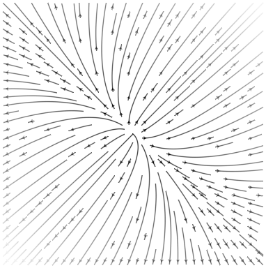
using Grassmann, Makie
basis"2" # Euclidean
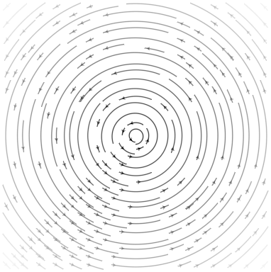
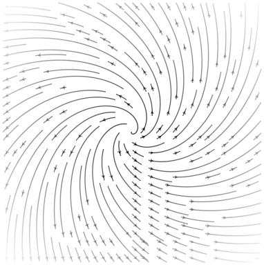
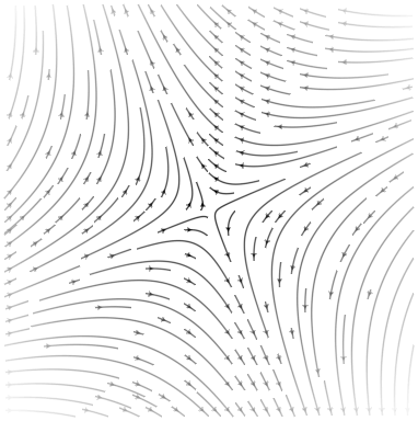
streamplot(vectorfield(exp(π*v12/2)),-1.5..1.5,-1.5..1.5)
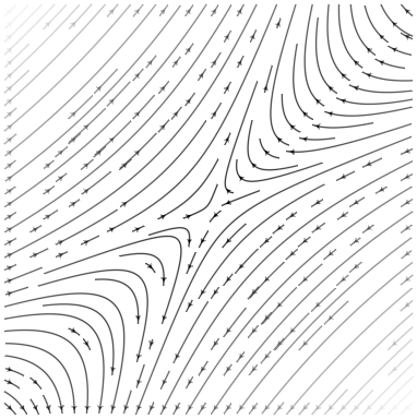
streamplot(vectorfield(exp((π/2)*v12/2)),-1.5..1.5,-1.5..1.5)
streamplot(vectorfield(exp((π/4)*v12/2)),-1.5..1.5,-1.5..1.5)
streamplot(vectorfield(v1*exp((π/4)*v12/2)),-1.5..1.5,-1.5..1.5)
@basis S"+-" # Hyperbolic
streamplot(vectorfield(exp((π/8)*v12/2)),-1.5..1.5,-1.5..1.5)
streamplot(vectorfield(v1*exp((π/4)*v12/2)),-1.5..1.5,-1.5..1.5)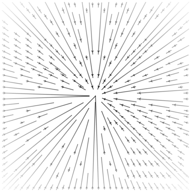

using Grassmann, Makie
@basis S"∞+++"
f(t) = (↓(exp(π*t*((3/7)*v12+v∞3))>>>↑(v1+v2+v3)))
lines(V(2,3,4).(points(f)))
@basis S"∞∅+++"
f(t) = (↓(exp(π*t*((3/7)*v12+v∞3))>>>↑(v1+v2+v3)))
lines(V(3,4,5).(points(f)))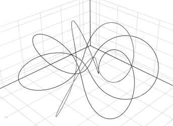

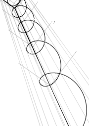
using Grassmann, Makie; @basis S"∞+++"
streamplot(vectorfield(exp((π/4)*(v12+v∞3)),V(2,3,4)),-1.5..1.5,-1.5..1.5,-1.5..1.5,gridsize=(10,10))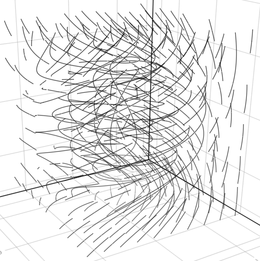

using Grassmann, Makie; @basis S"∞+++"
streamplot(vectorfield(exp((π/4)*(v12+v∞3)),V(2,3,4),V(1,2,3)),-1.5..1.5,-1.5..1.5,-1.5..1.5,gridsize=(10,10))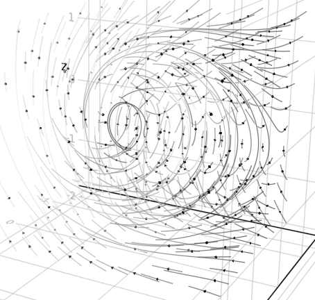

using Grassmann, Makie; @basis S"∞+++"
f(t) = ↓(exp(t*v∞*(sin(3t)*3v1+cos(2t)*7v2-sin(5t)*4v3)/2)>>>↑(v1+v2-v3))
lines(V(2,3,4).(points(f)))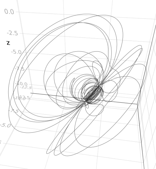

using Grassmann, Makie; @basis S"∞+++"
f(t) = ↓(exp(t*(v12+0.07v∞*(sin(3t)*3v1+cos(2t)*7v2-sin(5t)*4v3)/2))>>>↑(v1+v2-v3))
lines(V(2,3,4).(points(f)))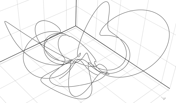

As a result of Grassmann's exterior & interior products, the Hodge-DeRahm chain complex from cohomology theory is

\[0 \,\underset{\partial}{\overset{d}{\rightleftarrows}}\, \Omega^0(M) \,\underset{\partial}{\overset{d}{\rightleftarrows}}\, \Omega^1(M) \,\underset{\partial}{\overset{d}{\rightleftarrows}}\, \cdots \,\underset{\partial}{\overset{d}{\rightleftarrows}}\, \Omega^n(M) \,\underset{\partial}{\overset{d}{\rightleftarrows}}\, 0,\]

having dimensional equivalence brought by the Grassmann-Hodge complement,

\[\mathcal H^{n-p}M \cong \frac{\text{ker}(d\Omega^{n-p}M)}{\text{im}(d\Omega^{n-p+1}M)}, \qquad \dim\mathcal H^pM = \dim\frac{\text{ker}(\partial\Omega^pM)}{\text{im}(\partial\Omega^{p+1}M)}.\]

The rank of the grade $p$ boundary incidence operator is

\[\text{rank}\langle\partial\langle M\rangle_{p+1}\rangle_p = \min\{\dim\langle\partial\langle M\rangle_{p+1}\rangle_p,\dim\langle M\rangle_{p+1}\}.\]

Invariant topological information can be computed using the rank of homology,

\[b_p(M) = \dim\langle M\rangle_{p+1} - \text{rank}\langle\partial\langle M\rangle_{p+1}\rangle_p - \text{rank}\langle\partial\langle M\rangle_{p+2}\rangle_{p+1}\]

are the Betti numbers with Euler characteristic $\chi(M) = \sum_p (-1)^pb_p$.

Let's obtain the full skeleton of a simplical complex $\Delta(\omega)=\mathcal P(\omega)\backslash\Lambda^0(V)$ from the power set $\mathcal P(\omega)$ of all vertices with each subcomplex $\Delta(\partial(\omega))$ contained in the edge graph:

\[\Delta(\omega) = \sum_{g=1}^n\sum_{k=1}^{n\choose g}\left(\text{abs}\langle\omega\rangle_{g,k} + \Delta\left(\text{abs}\,\partial\langle\omega\rangle_{g,k}\right)\right).\]

Compute the value $\chi(\Delta(\omega))=1$ and $\chi(\Delta(\partial(\omega))) = \, ?$ for any simplex $\omega$. As an exercise, also compute the corresponding betti numbers..

julia> [(χ(Δ(ω)),χ(Δ(∂(ω)))) for ω ∈ (Λ(ℝ5).v12,Λ(ℝ5).v123,Λ(ℝ5).v1234,Λ(ℝ5).v12345)]4-element Vector{Tuple{Int64, Int64}}:
 (1, 2)
 (1, 0)
 (1, 2)
 (1, 0)

These methods can be applied to any Multivector simplicial complex.

Null-basis of the projective split

Let $v_\pm^2 = \pm1$ be a basis with $v_\infty = v_++v_-$ and $v_\emptyset = (v_--v_+)/2$. An embedding space $\mathbb R^{p+1,q+1}$ carrying the action from the group $O(p+1,q+1)$ then has $v_\infty^2 =0$, $v_\emptyset^2 =0$, $v_\infty \cdot v_\emptyset = -1$, and $v_{\infty\emptyset}^2 = 1$ with Lobachevskian plane $v_{\infty\emptyset}$ having these product properties,

julia> using Grassmann; @basis S"∞∅++"(⟨∞∅11⟩, v, v∞, v∅, v₁, v₂, v∞∅, v∞₁, v∞₂, v∅₁, v∅₂, v₁₂, v∞∅₁, v∞∅₂, v∞₁₂, v∅₁₂, v∞∅₁₂)
julia> v∞^2, v∅^2, v1^2, v2^2(𝟎, 𝟎, 1v, 1v)
julia> v∞ ⋅ v∅, v∞∅^2(-1v, 1v)
julia> v∞∅ * v∞, v∞∅ * v∅(-1v∞, 1v∅)
julia> v∞ * v∅, v∅ * v∞(-1 + 1v∞∅ + 0v∞₁ + 0v∞₂ + 0v∅₁ + 0v∅₂ + 0v₁₂ + 0v∞∅₁₂, -1 - 1v∞∅ + 0v∞₁ + 0v∞₂ + 0v∅₁ + 0v∅₂ + 0v₁₂ + 0v∞∅₁₂)

For the null-basis, complement operations are different:

\[\star v_\infty = \star(v_++v_-) = (v_- + v_+)v_{1...n} = v_{\infty1...n}\]

\[ \star 2v_\emptyset = \star(v_--v_+) = (v_+ - v_-)v_{1...n} = -2v_{\emptyset1...n}\]

The Hodge complement satisfies $\langle\omega\ast\omega\rangle I=\omega\wedge\star\omega$. This property is naturally a result of using the geometric product in the definition. An additional metric independent version of the complement operation is available with the ! operator,

\[!v_\infty = !(v_++v_-) = (v_- - v_+)v_{1...n} = 2v_{\emptyset1...n}\]

\[!2v_\emptyset = !(v_--v_+) = (v_+ + v_-)v_{1...n} = -v_{\infty1...n}\]

For that variation of complement, $||\omega||^2 I = \omega\,\wedge\,!\omega$ holds.

julia> ⋆v∞, !v∞, ⋆v∅, !v∅(1v∞₁₂, 2v∅₁₂, -1v∅₁₂, -0.5v∞₁₂)
julia> !v∞ * v12 == -2v∅, !v∅ * v12 == v∞/2(true, true)
julia> ⋆v∞ * v12 == -v∞, ⋆v∅ * v12 == v∅(true, true)
julia> v∞ * !v∞, v∅ * !v∅(0 + 0v∞∅ + 0v∞₁ + 0v∞₂ + 0v∅₁ + 0v∅₂ - 2v₁₂ + 2v∞∅₁₂, -0.0 - 0.0v∞∅ - 0.0v∞₁ - 0.0v∞₂ - 0.0v∅₁ - 0.0v∅₂ + 0.5v₁₂ + 0.5v∞∅₁₂)

Extended tangent algebra basis

Definition (Symmetric Leibniz differentials): Let $\partial_k = \frac\partial{\partial x_k}\in L_gV\,$ be Leibnizian symmetric tensors, then there is an equivalence relation $\asymp$ which holds for each $\sigma\in S_p$

\[(\partial_p \circ \dots\circ \partial_1)\omega \asymp(\bigotimes_k \partial_{\sigma(k)})\omega \iff \ominus_k\partial_k = \bigodot_k\partial_k,\]

along with each derivation $\partial_k(\omega\eta) = \partial_k(\omega)\eta + \omega\partial_k(\eta)$.

The product rule is encoded into Grassmann algebra when a tangent bundle is used, demonstrated here symbolically with Reduce by using the dual number definition:

julia> using Grassmann, Reduce
Reduce (Free CSL version, revision 4590), 11-May-18 ...

julia> @mixedbasis tangent(ℝ^1)
(⟨+-₁¹⟩*, v, v₁, w¹, ϵ₁, ∂¹, v₁w¹, v₁ϵ₁, v₁∂¹, w¹ϵ₁, w¹∂¹, ϵ₁∂¹, v₁w¹ϵ₁, v₁w¹∂¹, v₁ϵ₁∂¹, w¹ϵ₁∂¹, v₁w¹ϵ₁∂¹)

julia> a,b = :x*v1 + :dx*ϵ1, :y*v1 + :dy*ϵ1
(xv₁ + dxϵ₁, yv₁ + dyϵ₁)

julia> a * b
x * y + (dy * x + dx * y)v₁ϵ₁

Higher order and multivariable Taylor numbers are also supported.

julia> @basis tangent(ℝ,2,2) # 1D Grade, 2nd Order, 2 Variables(T²⟨+₁₂⟩, v, v₁, ∂₁, ∂₂, ∂₁v₁, ∂₂v₁, ∂₁₂, ∂₁₂v₁)
julia> ∂1 * ∂1v1∂₁⊗∂₁v₁
julia> ∂1 * ∂2∂₁₂
julia> v1*∂12∂₁₂v₁
julia> ∂12*∂2 # 3rd order is zero𝟎
julia> @mixedbasis tangent(ℝ^2,2,2); # 2D Grade, 2nd Order, 2 Variables
julia> V(∇) # vector field0v₁₂ + 1∂₁v₁ + 0∂₂v₁ + 0∂₁v₂ + 1∂₂v₂ + 0∂₁₂
julia> V(∇) ⋅ V(∇) # Laplacian0 + 1∂₁⊗∂₁ + 1∂₂⊗∂₂
julia> ans*∂1 # 3rd order is zero0.0v⃖

Multiplication with an $\epsilon_i$ element is used help signify tensor fields so that differential operators are automatically applied in the Submanifold algebra as ∂ⱼ⊖(ω⊗ϵᵢ) = ∂ⱼ(ωϵᵢ) ≠ (∂ⱼ⊗ω)⊖ϵᵢ.

julia> using Reduce, Grassmann; @mixedbasis tangent(ℝ^2,3,2);

julia> (∂1+∂12) * (:(x1^2*x2^2)*ϵ1 + :(sin(x1))*ϵ2)
0.0 + (2 * x1 * x2 ^ 2)∂₁ϵ¹ + (cos(x1))∂₁ϵ² + (4 * x1 * x2)∂₁₂ϵ¹

Although fully generalized, the implementation in this release is still experimental.

Symbolic coefficients by declaring algebra

Due to the abstract generality of the code generation of the Grassmann product algebra, it is easily possible to extend the entire set of operations to other kinds of scalar coefficient types.

julia> using GaloisFields, Grassmann

julia> const F = GaloisField(7)
𝔽₇

julia> basis"2"
(⟨++⟩, v, v₁, v₂, v₁₂)

julia> F(3)*v1
3v₁

julia> inv(ans)
5v₁

By default, the coefficients are required to be <:Number. However, if this does not suit your needs, alternative scalar product algebras can be specified with

Grassmann.generate_algebra(:AbstractAlgebra,:SetElem)

where :SetElem is the desired scalar field and :AbstractAlgebra is the scope which contains the scalar field.

With the usage of Requires, symbolic scalar computation with Reduce.jl and other packages is automatically enabled,

julia> using Reduce, Grassmann
Reduce (Free CSL version, revision 4590), 11-May-18 ...

julia> basis"2"
(⟨++⟩, v, v₁, v₂, v₁₂)

julia> (:a*v1 + :b*v2) ⋅ (:c*v1 + :d*v2)
(a * c + b * d)v

julia> (:a*v1 + :b*v2) ∧ (:c*v1 + :d*v2)
0.0 + (a * d - b * c)v₁₂

julia> (:a*v1 + :b*v2) * (:c*v1 + :d*v2)
a * c + b * d + (a * d - b * c)v₁₂

If these compatibility steps are followed, then Grassmann will automatically declare the product algebra to use the Reduce.Algebra symbolic field operation scope.

julia> using Reduce,Grassmann; basis"4"
Reduce (Free CSL version, revision 4590), 11-May-18 ...
(⟨++++⟩, v, v₁, v₂, v₃, v₄, v₁₂, v₁₃, v₁₄, v₂₃, v₂₄, v₃₄, v₁₂₃, v₁₂₄, v₁₃₄, v₂₃₄, v₁₂₃₄)

julia> P,Q = :px*v1 + :py*v2 + :pz* v3 + v4, :qx*v1 + :qy*v2 + :qz*v3 + v4
(pxv₁ + pyv₂ + pzv₃ + 1.0v₄, qxv₁ + qyv₂ + qzv₃ + 1.0v₄)

julia> P∧Q
0.0 + (px * qy - py * qx)v₁₂ + (px * qz - pz * qx)v₁₃ + (px - qx)v₁₄ + (py * qz - pz * qy)v₂₃ + (py - qy)v₂₄ + (pz - qz)v₃₄

julia> R = :rx*v1 + :ry*v2 + :rz*v3 + v4
rxv₁ + ryv₂ + rzv₃ + 1.0v₄

julia> P∧Q∧R
0.0 + ((px * qy - py * qx) * rz - ((px * qz - pz * qx) * ry - (py * qz - pz * qy) * rx))v₁₂₃ + (((px * qy - py * qx) + (py - qy) * rx) - (px - qx) * ry)v₁₂₄ + (((px * qz - pz * qx) + (pz - qz) * rx) - (px - qx) * rz)v₁₃₄ + (((py * qz - pz * qy) + (pz - qz) * ry) - (py - qy) * rz)v₂₃₄

It should be straight-forward to easily substitute any other extended algebraic operations and fields; issues with questions or pull-requests to that end are welcome.